Analysis_Example
Analysis_Example.RmdIntroduction
In this document, we will demonstrate how to use the Survey-Embedded Carbon Footprint Calculator (SECFC) package. We will:
- Install the SECFC package from GitHub.
- Load SECFC and our sample dataset.
- Calculate carbon emissions using a built-in SECFC function.
- Run a linear regression to see how income predicts total carbon emissions.
- Create a plot of the data using ggplot2.
Step 1: Download the package from GitHub
First, we need to install the package from GitHub. If you do not have
remotes installed yet, run
install.packages("remotes") beforehand.
# Install the SECFC package from GitHub
remotes::install_github("jianing-d/SECFC")
#> cpp11 (NA -> 0.5.2) [CRAN]
#> ── R CMD build ─────────────────────────────────────────────────────────────────
#> * checking for file ‘/tmp/RtmpBsDwtz/remotes1b596296ce3a/jianing-d-SECFC-ecd1e8d/DESCRIPTION’ ... OK
#> * preparing ‘SECFC’:
#> * checking DESCRIPTION meta-information ... OK
#> * checking for LF line-endings in source and make files and shell scripts
#> * checking for empty or unneeded directories
#> * building ‘SECFC_0.1.0.tar.gz’
Step 2: Load the package
Load the SECFC package, which provides the
calc_total_emissions() function among others.
Step 3: Load your dataset
For demonstration, we assume you are use questionnaire_sample.rds that contains survey responses (provided and pre-loaded in our package).
# Replace the file path with your own dataset if necessary
questionnaire_example <- SECFC::questionnaire_example

required_cols <- c("SD_09_AdminCode")
missing_cols  <- setdiff(required_cols, names(questionnaire_example))
if (length(missing_cols)) {
  message("Adding missing columns: ", paste(missing_cols, collapse = ", "))
  questionnaire_example[missing_cols] <- NA_character_
}


# Take a quick look at your data structure
str(questionnaire_example)
#> tibble [50 × 36] (S3: tbl_df/tbl/data.frame)
#>  $ RecordedDate          : chr [1:50] "30/6/2024 22:38" "30/6/2024 22:39" "30/6/2024 22:40" "30/6/2024 22:40" ...
#>  $ T_01_CarUsage         : num [1:50] 4 3 3 4 5 4 5 4 3 3 ...
#>  $ T_02_CarType          : chr [1:50] "Hybrid Vehicle" "Hybrid Vehicle" "Diesel Vehicle" "Hybrid Vehicle" ...
#>  $ T_03_CarDistance      : num [1:50] 2 1 3 2 2 3 4 1 4 2 ...
#>  $ T_04_PublicTransport  : num [1:50] 5 4 5 4 4 5 5 5 5 4 ...
#>  $ T_05_PublicTransport  : num [1:50] 4 4 4 2 4 4 4 4 4 1 ...
#>  $ T_06_AirTravelLong    : num [1:50] 2 1 1 1 1 4 2 1 1 1 ...
#>  $ T_07_AirTravelShort   : chr [1:50] "7-10 flights" "More than 10 flights" "4-6 flights" "More than 10 flights" ...
#>  $ T_08_LongDistanceTra  : num [1:50] 5 4 5 4 4 5 5 5 5 5 ...
#>  $ PETS_4                : num [1:50] 0 0 4 1 5 1 1 0 0 1 ...
#>  $ PETS_5                : num [1:50] 2 0 2 1 1 1 0 0 0 0 ...
#>  $ E1_Electricity Usage  : num [1:50] 2 2 2 1 1 1 1 4 1 1 ...
#>  $ EH_02_ElectricityBil_1: num [1:50] 300 79 153 73 107 181 80 130 132 27 ...
#>  $ EH_05_NaturalGasBill_1: num [1:50] 59 46 0 27 47 20 0 80 0 27 ...
#>  $ EH_07_WaterBill       : num [1:50] 119 0 35 0 17 25 40 0 80 150 ...
#>  $ F_01_DietaryHabits_5  : num [1:50] 12 8 6 9 10 1 7 8 13 8 ...
#>  $ F_01_DietaryHabits_6  : num [1:50] 0 0 2 0 4 0 0 0 1 1 ...
#>  $ F_01_DietaryHabits_7  : num [1:50] 0 2 0 1 4 0 5 0 5 2 ...
#>  $ F_01_DietaryHabits_4  : num [1:50] 5 5 3 7 11 7 2 14 7 8 ...
#>  $ CL_01_ClothingPurcha  : num [1:50] 3 3 4 3 4 3 4 5 3 3 ...
#>  $ CL_03_MonthlyEx_9     : num [1:50] 0 15 200 20 0 0 200 0 0 0 ...
#>  $ CL_03_MonthlyEx_10    : num [1:50] 200 100 0 49 0 150 100 100 250 100 ...
#>  $ CL_03_MonthlyEx_11    : num [1:50] 200 0 0 58 0 100 0 0 0 0 ...
#>  $ CL_03_MonthlyEx_12    : num [1:50] 0 0 0 0 100 100 0 0 0 0 ...
#>  $ CL_03_MonthlyEx_13    : num [1:50] 30 25 0 20 100 500 0 0 0 0 ...
#>  $ CL_03_MonthlyEx_14    : num [1:50] 50 35 50 0 0 80 50 100 100 100 ...
#>  $ CL_03_MonthlyEx_15    : num [1:50] 0 0 35 150 0 610 0 800 0 0 ...
#>  $ SD_06_HouseholdSize_17: num [1:50] 4 1 1 2 4 4 1 2 2 1 ...
#>  $ SD_06_HouseholdSize_18: num [1:50] 0 0 0 1 0 2 0 2 0 0 ...
#>  $ SD_06_HouseholdSize_19: num [1:50] 0 0 0 0 2 2 0 0 0 0 ...
#>  $ SD_07_Country         : chr [1:50] "China" "China" "China" "China" ...
#>  $ SD_08_ZipCode         : chr [1:50] NA NA NA NA ...
#>  $ EH_03_ElectricityBil_1: num [1:50] 3600 948 1836 876 1284 ...
#>  $ EH_06_NaturalGasBill_1: num [1:50] 708 552 0 324 564 240 0 960 0 324 ...
#>  $ income                : num [1:50] 70011 42460 38100 55435 46043 ...
#>  $ SD_09_AdminCode       : chr [1:50] "410000" "320000" "110000" "370000" ...
Step 4: Calculate total carbon emissions
Now we use the calc_total_emissions() function from
SECFC to estimate each respondent’s carbon footprint based on their
survey responses. A new data frame, questionnaire_example_total, is now
available in your R environment. It has several new variables, including
TotalEmissions, the individual respondent’s overall estimated
footprint.
calc_total_emissions(questionnaire_example)
#> # A tibble: 50 × 45
#>    RecordedDate T_01_CarUsage T_02_CarType T_03_CarDistance T_04_PublicTransport
#>    <chr>                <dbl> <chr>                   <dbl>                <dbl>
#>  1 30/6/2024 2…           5.5 Hybrid Vehi…             10                      5
#>  2 30/6/2024 2…           3.5 Hybrid Vehi…              5                      4
#>  3 30/6/2024 2…           3.5 Diesel Vehi…             30.5                    5
#>  4 30/6/2024 2…           5.5 Hybrid Vehi…             10                      4
#>  5 30/6/2024 2…           7   Hybrid Vehi…             10                      4
#>  6 30/6/2024 2…           5.5 Hybrid Vehi…             30.5                    5
#>  7 30/6/2024 2…           7   Hybrid Vehi…             51                      5
#>  8 30/6/2024 2…           5.5 Hybrid Vehi…              5                      5
#>  9 30/6/2024 2…           3.5 Diesel Vehi…             51                      5
#> 10 30/6/2024 2…           3.5 Hybrid Vehi…             10                      4
#> # ℹ 40 more rows
#> # ℹ 40 more variables: T_05_PublicTransport <dbl>, T_06_AirTravelLong <dbl>,
#> #   T_07_AirTravelShort <dbl>, T_08_LongDistanceTra <dbl>, PETS_4 <dbl>,
#> #   PETS_5 <dbl>, `E1_Electricity Usage` <dbl>, EH_02_ElectricityBil_1 <dbl>,
#> #   EH_05_NaturalGasBill_1 <dbl>, EH_07_WaterBill <dbl>,
#> #   F_01_DietaryHabits_5 <dbl>, F_01_DietaryHabits_6 <dbl>,
#> #   F_01_DietaryHabits_7 <dbl>, F_01_DietaryHabits_4 <dbl>, …

# Check the first few rows
head(questionnaire_example_total)
#> # A tibble: 6 × 45
#>   RecordedDate  T_01_CarUsage T_02_CarType T_03_CarDistance T_04_PublicTransport
#>   <chr>                 <dbl> <chr>                   <dbl>                <dbl>
#> 1 30/6/2024 22…           5.5 Hybrid Vehi…             10                      5
#> 2 30/6/2024 22…           3.5 Hybrid Vehi…              5                      4
#> 3 30/6/2024 22…           3.5 Diesel Vehi…             30.5                    5
#> 4 30/6/2024 22…           5.5 Hybrid Vehi…             10                      4
#> 5 30/6/2024 22…           7   Hybrid Vehi…             10                      4
#> 6 30/6/2024 22…           5.5 Hybrid Vehi…             30.5                    5
#> # ℹ 40 more variables: T_05_PublicTransport <dbl>, T_06_AirTravelLong <dbl>,
#> #   T_07_AirTravelShort <dbl>, T_08_LongDistanceTra <dbl>, PETS_4 <dbl>,
#> #   PETS_5 <dbl>, `E1_Electricity Usage` <dbl>, EH_02_ElectricityBil_1 <dbl>,
#> #   EH_05_NaturalGasBill_1 <dbl>, EH_07_WaterBill <dbl>,
#> #   F_01_DietaryHabits_5 <dbl>, F_01_DietaryHabits_6 <dbl>,
#> #   F_01_DietaryHabits_7 <dbl>, F_01_DietaryHabits_4 <dbl>,
#> #   CL_01_ClothingPurcha <dbl>, CL_03_MonthlyEx_9 <dbl>, …
Step 5: Run a linear regression
We will examine how a respondent’s income might predict their total
carbon emissions. This is a basic linear model using the built-in
lm() function.
model <- lm(TotalEmissions ~ income, data = questionnaire_example_total)

# Display summary statistics of the regression
summary(model)
#>
#> Call:
#> lm(formula = TotalEmissions ~ income, data = questionnaire_example_total)
#>
#> Residuals:
#>     Min      1Q  Median      3Q     Max
#> -3681.4 -1829.0   171.2  1823.4  4032.0
#>
#> Coefficients:
#>              Estimate Std. Error t value Pr(>|t|)
#> (Intercept) 7.091e+03  6.486e+02   10.93 1.26e-14 ***
#> income      3.223e-02  9.424e-03    3.42  0.00129 **
#> ---
#> Signif. codes:  0 '***' 0.001 '**' 0.01 '*' 0.05 '.' 0.1 ' ' 1
#>
#> Residual standard error: 2093 on 48 degrees of freedom
#> Multiple R-squared:  0.1959, Adjusted R-squared:  0.1792
#> F-statistic:  11.7 on 1 and 48 DF,  p-value: 0.001286
Step 6: Create a Plot
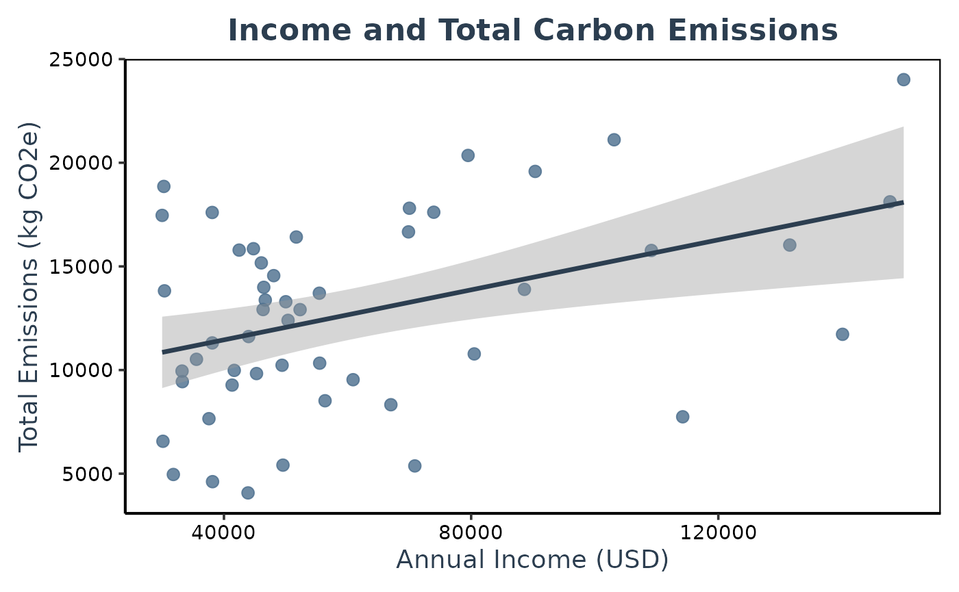
Finally, we can visualize the relationship between income and
TotalEmissions using ggplot2. The plot below includes:
- Points representing individual respondents
- A linear regression line (and confidence interval)
# Load ggplot2
library(ggplot2)

# Define custom colors
point_color <- "#4A6D8C"  # desaturated blue-grey for points
line_color  <- "#2C3E50"  # deeper blue-grey for the regression line

lm_plot <- ggplot(questionnaire_example_total, aes(x = income, y = TotalEmissions)) +
  geom_point(color = point_color, size = 2.8, alpha = 0.8) +
  geom_smooth(method = "lm", se = TRUE, color = line_color, linewidth = 1.2) +
  labs(
    title = "Income and Total Carbon Emissions",
    x = "Annual Income (USD)",
    y = "Total Emissions (kg CO2e)"
  ) +
  theme_classic(base_size = 14) +
  theme(
    plot.title   = element_text(face = "bold", hjust = 0.5, color = line_color),
    axis.title   = element_text(color = line_color),
    axis.text    = element_text(color = "black"),
    panel.border = element_rect(color = "black", fill = NA, linewidth = 0.8),
    plot.margin  = margin(10, 10, 10, 10)
  )

# Print the plot
lm_plot